Image Plots
At any point in the Virtual Pipeline the val of the FC_objects
of dimension
- 3D (x, y, wav)
- 2D (x, y)
can be visualized by using
to plot
- a image slice of the entire
- the entire
image, respectively.
The method plots the FC_object.val (3D) close to a certain requested wav_interest. Since in a FC_object.val (2D) has only one entry in wav, wav_interest is not necessary.
One of the plotting modes has to be chosen:
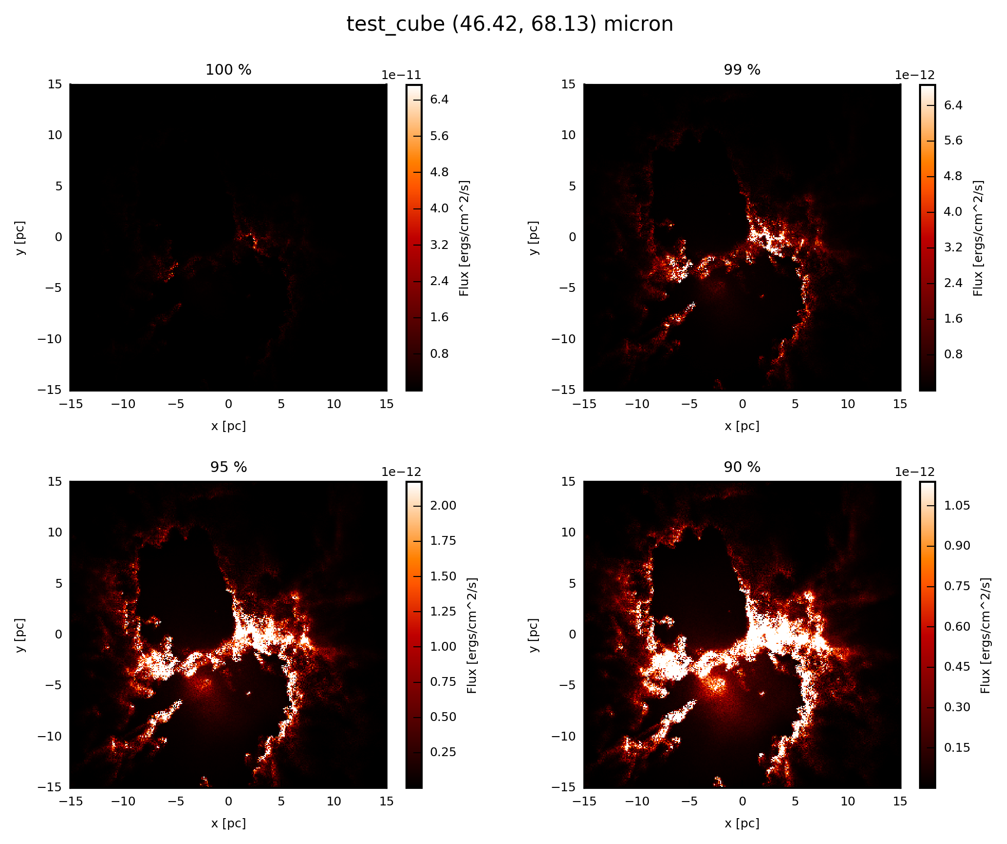
multi_cut:- Will plot the selected image at four cuts [100, 99, 95, 90]%.
Default is
Noneand enable withTrue.
single_cut:- Will plot the selected image at a selected cut between [0, 100]%.
Default is
Noneand enable with e.g80..
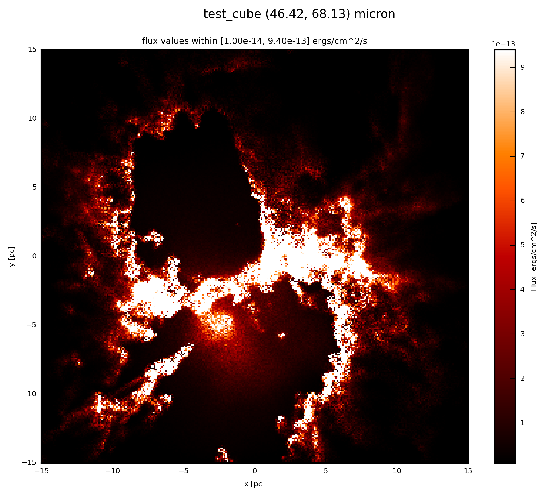
set_cut:- Will plot the selected image within an upper and lower cut in the
unitsof theval. Default isNoneand enable with range e.g(1e-14,9.4e-13).
To disable the different modes put None in the respected input parameters.
Of course you can plot different modes at the same time.
With prefix you can choose your own name for the plotted image (e.g. prefix.png).
Note
If prefix is enabled, only one plotting parameter can be chosen to prevent overplotting. If the default naming chain is enabled (prefix=None), more than one plotting mode can be chosen.
name is a part of the name of the output file (e.g. FC_object.name``_image_``plot_*.png). Where * stands for the modes and the wavelength interval within plotting.
Note
If prefix is enabled, name is not required and hence its default is None.
You also can adjust the resolution with dpi.
For further information see:
Example: Plot
If the FC_object is a SyntheticCube you can produce an image output at wav_interest = 60. in all modes, by adding to your script:
# plot FC_object.val (3D) at 60 microns with default naming
FC_object.plot_image(name='plot', wav_interest=60., set_cut=(1e-14,
                     9.4e-13), single_cut=80., multi_cut=True, dpi=300)

# plot FC_object.val (3D) at 60 microns with prefix
FC_object.plot_image(prefix='prefix1', wav_interest=60., multi_cut=True,
                     dpi=300)
FC_object.plot_image(prefix='prefix2', wav_interest=60., set_cut=(1e-14,
                     9.4e-13), dpi=300)
FC_object.plot_image(prefix='prefix3', wav_interest=60., single_cut=80.,
                     dpi=300)
In the default naming case you will find the files
FC_object.name_image_plot_multi_cut_46.42_68.13.pngFC_object.name_image_plot_set_cut_1.00e-14_9.40e-13_46.42_68.13.pngFC_object.name_image_plot_single_cut_80.0%_46.42_68.13.png
and in the prefix case you will find the files
prefix1.pngprefix2.pngprefix3.png
in the same directory as example.py. If you extend the example described in SyntheticCube, the resulting image will be exactly the same as displayed below.

If the FC_object is a SyntheticImage, because it was already convolved with a filter before, you plot with the following:
# plot FC_object.val (2D) at FC_object.wav
FC_object.plot_image(name='plot', set_cut=(1e-14, 9.4e-13), single_cut=80.,
                     multi_cut=True, dpi=300)

# plot FC_object.val (2D) at FC_object.wav with prefix
FC_object.plot_image(prefix='prefix1',  multi_cut=True, dpi=300)
FC_object.plot_image(prefix='prefix2',  set_cut=(1e-14, 9.4e-13), dpi=300)
FC_object.plot_image(prefix='prefix3',  single_cut=80., dpi=300)
In the default naming case you will find the files
FC_object.name_image_plot_multi_cut_*.pngFC_object.name_image_plot_set_cut_1.00e-14_9.40e-13_*.pngFC_object.name_image_plot_single_cut_80.0%_*.png
and in the prefix case you will find the files
prefix1.pngprefix2.pngprefix3.png
in the same directory as example.py, where * stands for the filter limits.