SyntheticCube

To start with a 3D image group from the Hyperion output your Python script example.py should contain:

import numpy as np

from hyperion.model import ModelOutput
from hyperion.util.constants import kpc
from fluxcompensator.cube import *

# read in from Hyperion
m = ModelOutput('hyperion_output.rtout')
array = m.get_image(group=0, inclination=0, distance=10*kpc,
                    units='ergs/cm^2/s')

Now your image (from image group=0 starting from 0, which contains an image in this example) is scaled to 300 pc in units of 'ergs/cm^2/s'. For further details see ModelOutput.

See also

You can download an example output (density input from Dale et al. 2012) from here: ../../fluxcompensator/tests/hyperion_output.rtout

To start with the FluxCompensator class SyntheticCube, you simlpy write:

# initial FluxCompensator array
FC_object = SyntheticCube(input_array=array, unit_out='ergs/cm^2/s',
                          name='test_cube')

The output unit of the FluxCompensator unit_out can be defined. Possible are all units like in get_image. unit_out='ergs/cm^2/s' is the default. The name of the FluxCompensator run name can be defined with a str. All outputs (e.g. plots) will start with this name by default.

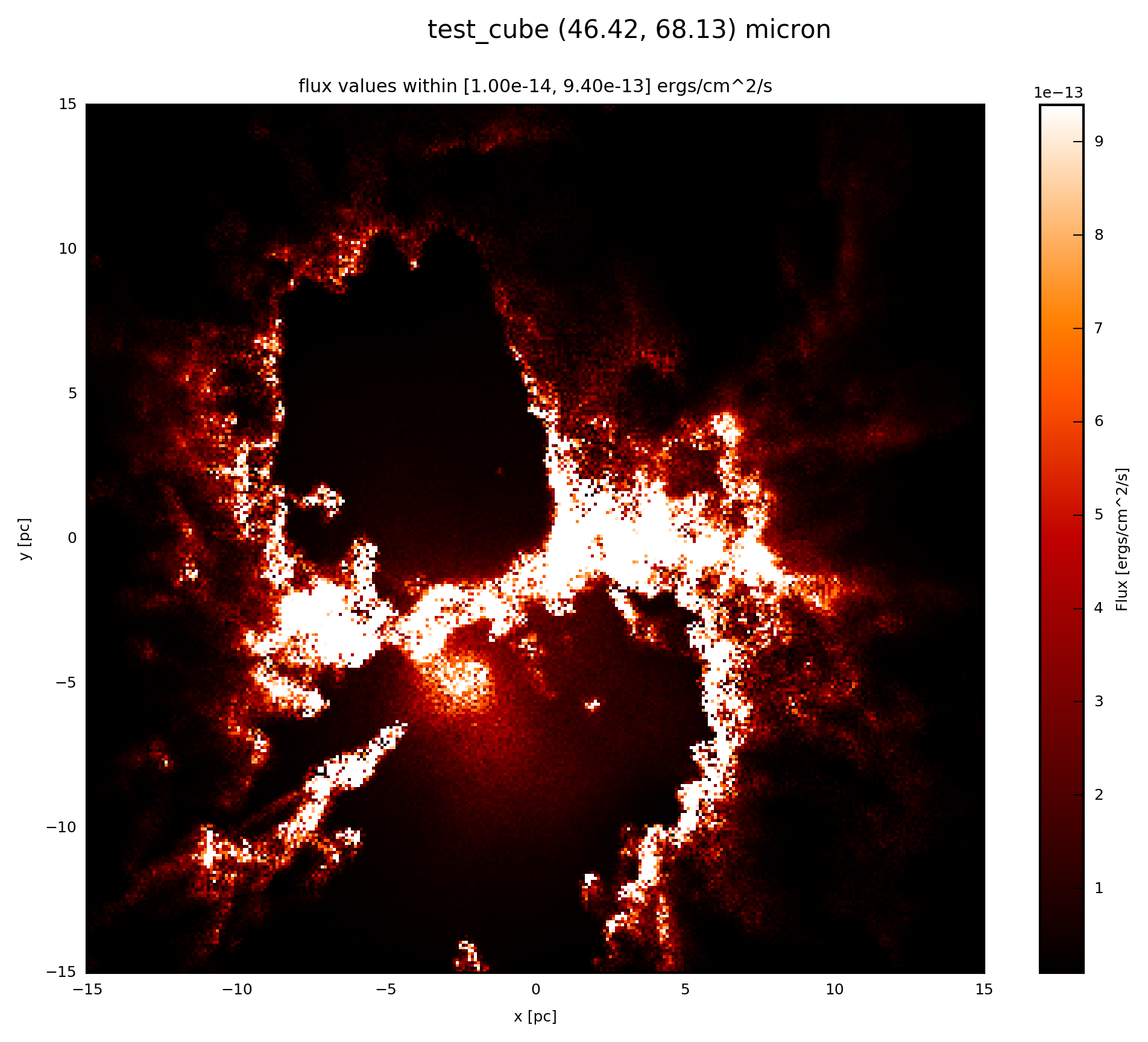
You will produce an image output if you follow the instructions Image Plots or by adding to your script:

# plot FC_object.val at 60 microns
FC_object.plot_image(name='init', wav_interest=60., set_cut=(1e-14, 9.4e-13),
             single_cut=None, multi_cut=None, dpi=300)

In this case you will find the file test_cube_image_init_set_cut_1.00e-14_9.40e-13_46.42_68.13.png in the same directory as example.py.