Extiction
Accounting for reddening is essential when making synthetic observations more realistic. The FluxCompensator enables the user to use its own extinction law or to derred with the law provided by the FluxCompensator.
In any case the methods
fluxcompensator.cube.SyntheticCube.extinction()fluxcompensator.image.SyntheticImage.extinction()fluxcompensator.sed.SyntheticSED.extinction()fluxcompensator.flux.SyntheticFlux.extinction()
will derred the physical properties val of dimensions
- 3D (x, y, wav)
- 2D (x, y)
- 1D (wav)
- 0D (wav)
of the different FC_objects.
First, for all wavelengths the opacity \(k_\lambda\) will be interpolated. Afterwards the wavelength dependent extinction \(A_\lambda\) will be calculated with the given visual opacity \(k_V\) (e.g. \(k_V = 211.4 cm^2/g\) for the law used here):
Now val can be deredded:
Use Own Extinction Law
If you want to use your own extinction law you need to prepare an file (e.g. my_extinction.txt) with 2 columns. In column 1 write the wavelength in microns and in column 2 write the opacity in cm^2/g.
Furthermore you need to interpolate the opacity k_v at 0.550 microns (e.g. k_v = 200. ).
Now derred a passed FC_objects with your extinction law by adding to your script:
# dered with own extinction law
ext = FC_object.extinction(A_v=20., input_opacities='my_extinction.txt',
                           k_v=200.)
Built-in Extinction Law
The extinction law provided here is from Kim et al. 1994 (the law used in the SED fitting tool published in Robitaille et al. (2007). For further infomation see http://caravan.astro.wisc.edu/protostars/.
Note
Note that this extinction law breaks down above 1 mm and below 0.02 microns.
Now derred a passed FC_objects with the built-in extinction law by adding to your script:
# dered with provided extinction law
ext = FC_object.extinction(A_v=20.)
Example: Plot
If the FC_object is a SyntheticCube, you can produce an image output by following the instruction Image Plots.
The essentials are given here; add to your script:
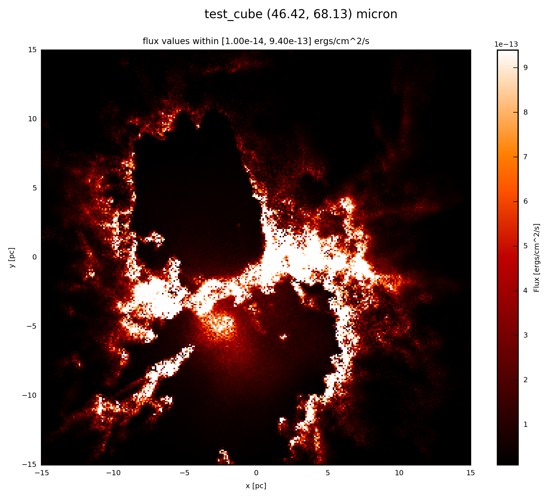
# plot ext.val (3D) at 60 microns
ext.plot_image(name='ext', wav_interest=60., set_cut=(1e-14, 9.4e-13),
               single_cut=None, multi_cut=None, dpi=300)
In this case you will find the file test_cube_image_ext_set_cut_1.00e-14_9.40e-13_46.42_68.13.png in the same directory as example.py. If you extend the example described in SyntheticCube, the resulting image will be exactly the same as displayed below.
If the FC_object is a SyntheticImage, because it was already convolved with a filter before, you plot with the following:
# plot ext.val (2D) at ext.wav
ext.plot_image(name='ext', set_cut=(1e-14, 9.4e-13), single_cut=None,
               multi_cut=None, dpi=300)
In this case you will find the file test_cube_image_ext_set_cut_1.00e-14_9.40e-13_*.png in the same directory as example.py, where * stands for the filter limits.