Convolve with Filters
As in a normal telescope at some point you might want to select a certain wavelength. In telescopes this can be achieved by using filters. Here we need to convolve the synthetic measurements with a filter function.
With
fluxcompensator.cube.SyntheticCube.convolve_filter()fluxcompensator.sed.SyntheticSED.convolve_filter()
you can convolve a synthetic measurement val of
- 3D (x, y, wav)
- 1D (wav)
dimension in the different FC_objects, respectively, within a certain wavelength bin. After the convolution an
- image
SyntheticImage - photometric val
SyntheticFlux
remains, respectively, for a certain band.
To initialize the convolution add to you script:
# convolve with filter object
filtered = FC_object.convolve_filter(filter_input, plot_rebin=None,
                                     plot_rebin_dpi=None)
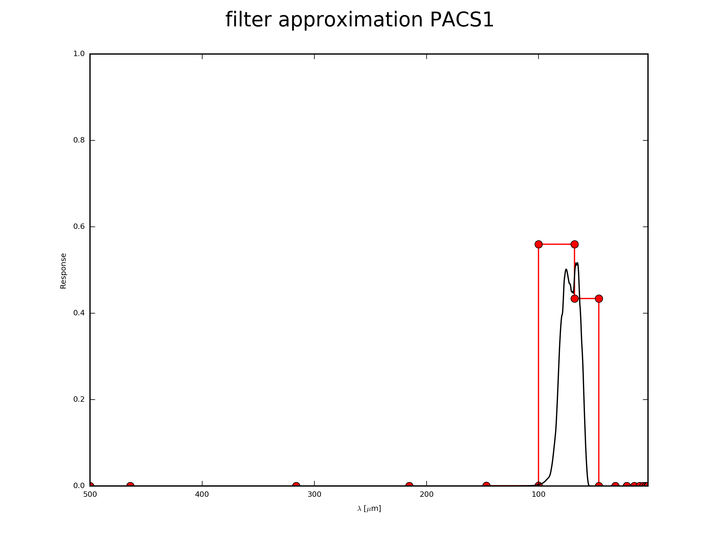
filter_input can be either your own filter function or a function from the Database of routinely applied detectors. plot_rebin=True plots the initial filter response and the new response after rebinning. With plot_rebin_dpi one can adjust the resolution of the plot. If you use the PACS1 filter PACS1_FILTER from the Database (see below), you produce the following plot of the rebinning:
# convolve with filter object
filtered = FC_object.convolve_filter(filter_input, plot_rebin=True,
                                     plot_rebin_dpi=300)
In this case you will find the file test_cube_process-output_FR-PACS1-rebin.png in the same directory as example.py. If you extend the example described in SyntheticCube, the resulting plot will be exactly the same as displayed below.
Arbitrary Filter Function
If you have your own filter function in a file with 2 columns (e. g filter.txt). Column 1 contains the wavelength in microns and column 2 contains the filter response:
# wav [microns]     response
3.1                 0.0
3.0                 0.3
2.0                 0.3
1.9                 0.0
Further information of the filter is needed:
- central wavelength of the filter
waf_0 alphaval of filterbetaval of filter
alpha represents the exponent in the power law if
beta represents the exponent in the power law if
If the input of the response in column 2 is in ...
- unit energy –>
beta=-1 - unit photon –>
beta=0
For a detailed description see Robitaille et al. (2007, Appendix) and Koepferl & Robitaille (subm. to ApJ).
Now to define your own filter, add the following to you script:
from fluxcompensator.filter import Filter

# create own filter object
filter_input = Filter(name='my_filter', filter_file='filter.txt',
                      waf_0=2.5, alpha=1, beta=0)
Database Filter Function
The FluxCompensator contains 24 routinely applied filters from 2MASS, SPITZER, HERSCHEL, WISE and IRAS in its Database. If you want to use this predefined filter objects (e.g. PACS1_FILTER), add the following to your script:
import fluxcompensator.database.missions as filters

# call object from the filter database
filter_input = getattr(filters, 'PACS1_FILTER')
The filter objects in the Database (e.g. PACS1_FILTER) can be called by using getattr and the str of the filter object.
Possible names of the attributes are:
filter            waf_0     waf_min        waf_max      alpha   beta

J_2MASS_FILTER            1.235     1.062          1.450          1       0
H_2MASS_FILTER            1.662     1.289          1.914          1       0
K_2MASS_FILTER            2.159     1.900          2.399          1       0

IRAC1_FILTER              3.550     3.081060       4.010380       1       0
IRAC2_FILTER              4.493     3.722490       5.221980       1       0
IRAC3_FILTER              5.731     4.744210       6.622510       1       0
IRAC4_FILTER              7.872     6.151150      10.496800       1       0

MIPS1_FILTER     23.68     18.005         32.207         -2      -1
MIPS2_FILTER            71.42      49.95998      111.0222        -2      -1
MIPS3_FILTER           155.9      100.0851       199.92          -2      -1

IRAS1_FILTER             12.        7.0           15.5            1      -1
IRAS2_FILTER             25.       16.0           31.5            1      -1
IRAS3_FILTER             60.       27.0           87.0            1      -1
IRAS4_FILTER            100.       65.0          140.0            1      -1

PACS1_FILTER             70.       48.72109985   157.47999573     1       0
PACS2_FILTER            100.       48.95959854   186.91600037     1       0
PACS3_FILTER            160.      105.26300049   500.00000000     1       0

SPIRE1_FILTER           250.      115.01458      291.41095       -2      -1
SPIRE2_FILTER           350.      137.39661      419.45077       -2      -1
SPIRE3_FILTER           500.      316.42866      603.04174       -2      -1

WISE1_FILTER              3.3526    2.53           6.50           2       0
WISE2_FILTER              4.6028    2.53           8.00           2       0
WISE3_FILTER             11.5608    2.53          28.55           2       0
WISE4_FILTER             22.0883    2.53          28.55           2       0
For a list of filter references see Koepferl & Robitaille (subm. to ApJ).
For further information see:
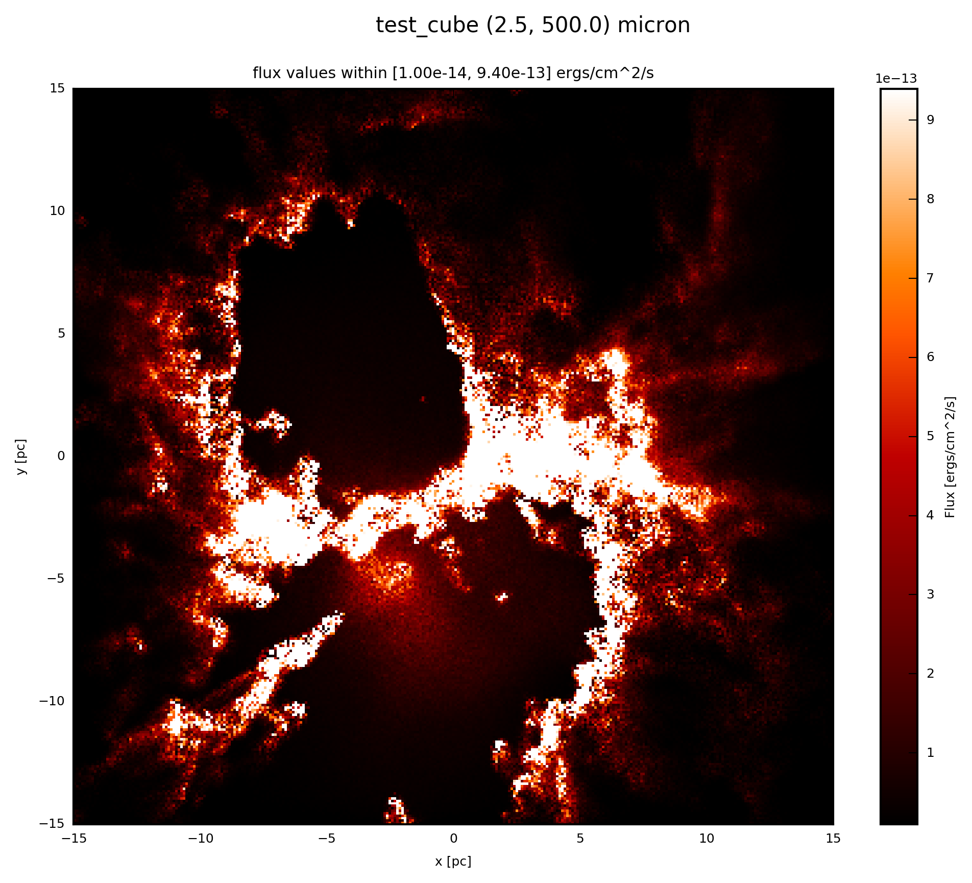
Example: Plot
If the FC_object is a SyntheticCube, you can produce an image output by following the instruction Image Plots.
The essentials are given here; add to your script:
# plot filtered.val (3D)
filtered.plot_image(name='filter', set_cut=(1e-14, 9.4e-13),
                    single_cut=None, multi_cut=None, dpi=300)
In this case you will find the file test_cube_image_filter_set_cut_1.00e-14_9.40e-13_2.5_500.0.png in the same directory as example.py. If you extend the example described in SyntheticCube, the resulting image will be exactly the same as displayed below.