SED Plots¶

At any point in the Virtual Pipeline you can plot a SyntheticFlux FC_object of 0D (wav) dimension created by

convolve_filter

with a SyntheticSED FC_object of 1D (wav) dimension from

in one plot.

Plot SyntheticFlux Value with SED¶

To plot 0D val passed by a FC_object f with a certain 1D SED s you can do this with fluxcompensator.flux.SyntheticFlux.plot_sed_filter(). Add to your script:

# plot f.val with s.val in one plot
f.plot_sed_filter(wav_sed=s.wav, rough_sed=s.val, ymin=1.e-5, dpi=300)

With ymin you can adjust the minimum val of the vertical axis. With dpi you can change the resolution of the plot. The output you will find in the file FC_object.name _process-output_SF- FC_object.fiter['name'] .png in the same directory as example.py.

Note

Here s does not necessarily must to be a member of FC_object but it needs to be a 1D numpy array.

If you extend the example described in SyntheticCube, to get FC_object f as the example in convolve_filter and the FC_object s as the example in get_rough_sed

from hyperion.model import ModelOutput
from hyperion.util.constants import kpc
from fluxcompensator.cube import *


# read in from Hyperion
m = ModelOutput('hyperion_output.rtout')
array = m.get_image(group=0, inclination=0, distance=10*kpc,
                    units='ergs/cm^2/s')

# initial FluxCompensator array
FC_object = SyntheticCube(input_array=array, unit_out='ergs/cm^2/s',
                  name='test_cube')

# collapse 3D cube to rough SED
FC_object_s = FC_object.get_rough_sed()

import fluxcompensator.database.missions as filters

# call object from the filter database
filter_input = getattr(filters, 'PACS1_FILTER')

# convolve with filter object
filtered = FC_object.convolve_filter(filter_input, plot_rebin=None,
                                     plot_rebin_dpi=None)

# collapse filtered.val
FC_object_f = filtered.get_total_val()

# plot single flux value and SED in one plot
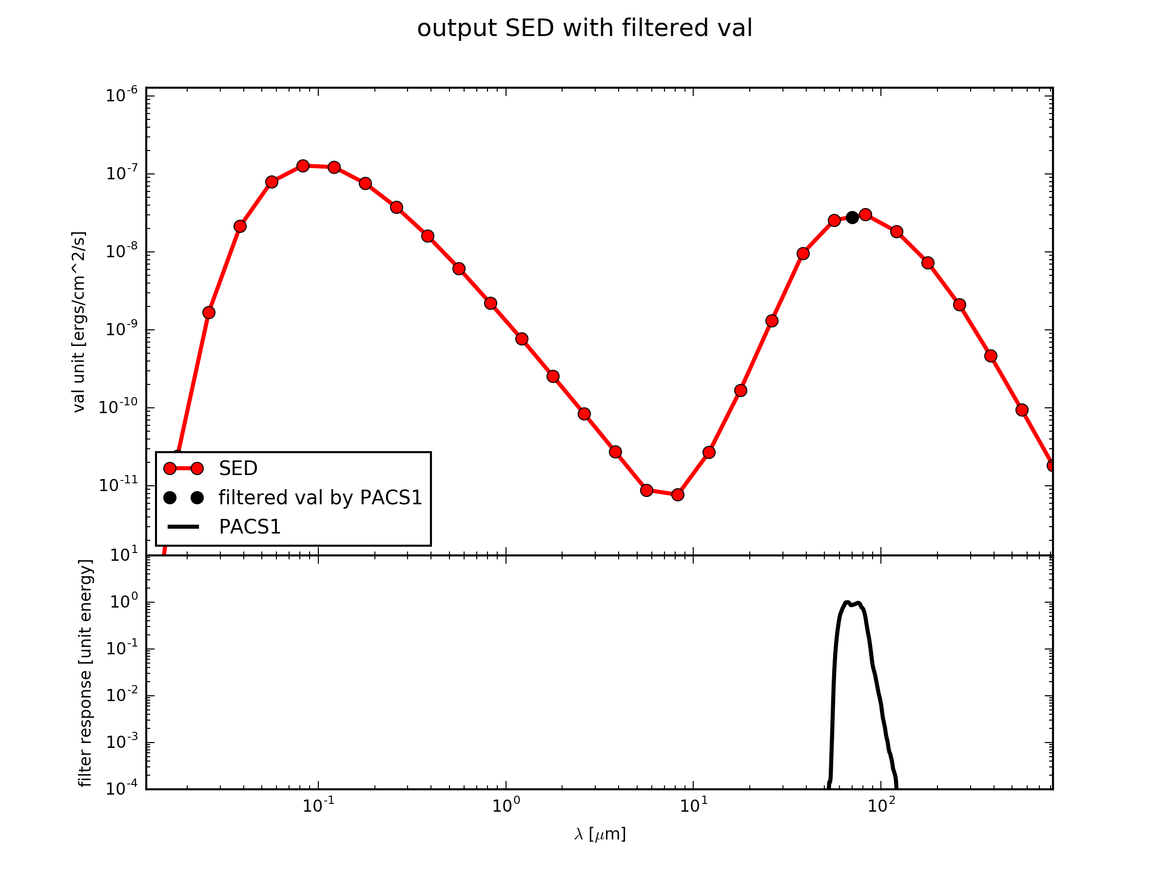
FC_object_f.plot_sed_filter(wav_sed=FC_object_s.wav, val_sed=FC_object_s.val, ymin=1.e-5, dpi=300)

the plot test_cube_process-output_SF-PACS1.png will be exactly the same like the following.

../_images/test_cube_process-output_SF-PACS1.png

Plot Many Fluxes with SED¶

At some point you might want to loop over many filters and you might have many 0D val which you compare to a SED in a plot. To do so, you save all the different 0D val of SyntheticFlux in an array (e.g. val_array) and you also have to store the wavelength of the filters in wav_array and their names in name_array.

To plot those arrays with the SED s with the fluxcompensator.sed.SyntheticSED.plot_sed_multi_filter() by adding to you script:

# plot all filters in loop with filtered val and rough_sed
FC_object_s.plot_sed_multi_filter(multi_filter_val=val_array,
                        multi_filter_wav=wav_array, names=filter_array,
                        ymin=1e-5, filter_label_size=None, dpi=300)

With ymin you can adjust the minimum val of the vertical axis. With dpi you can change the resolution of the plot. If filter_label_size=True the name of the filters are printed in a small font size. If you want to adjust the size just replace True with a number.

You will find the output file FC_object.name _process-output_SS-multi-filter.png in the same directory as example.py.

For further information see the tutorials of Multi-filter-Plot.