Multi-filter-Plot

As in SED Plots discribed you can loop over many filters (e.g. all the filters from the Database) and plot the resulting photometric flux together with the some SED (e.g. rough_SED from the initial 3D cube set-up).

Here is an example how to do that:

import numpy as np

from hyperion.model import ModelOutput
from hyperion.util.constants import kpc
from fluxcompensator.cube import *


# read in from Hyperion
m = ModelOutput('hyperion_output.rtout')
array = m.get_image(group=0, inclination=0, distance=10*kpc,
                    units='ergs/cm^2/s')

# initial FluxCompensator array
c = SyntheticCube(input_array=array, unit_out='ergs/cm^2/s',
                  name='test_cube')

# collapse 3D cube to rough SED
s = c.get_rough_sed()

import fluxcompensator.database.missions as filters

# empty arrays for storage
val_array = np.array(())
wav_array = np.array(())
filter_array = np.array(())

for loop_filter in ['J_2MASS', 'H_2MASS', 'K_2MASS', 'IRAS1', 'IRAS2',
                    'IRAS3', 'IRAS4','IRAC1', 'IRAC2', 'IRAC3', 'IRAC4',
                    'MIPS1', 'MIPS2', 'MIPS3','WISE1', 'WISE2', 'WISE3',
                    'WISE4', 'PACS1', 'PACS2', 'PACS3', 'SPIRE1', 'SPIRE2',
                    'SPIRE3']:

    # call object from the filter database
    filter_input = getattr(filters, loop_filter + '_FILTER')

    # convolve with filter object
    filtered = c.convolve_filter(filter_input, plot_rebin=None,
                                 plot_rebin_dpi=None)

    # collapse FC_object.val
    f = filtered.get_total_val()

    # store f.val, f.wav and filter_input in arrays
    # for plot_sed_multi_filter()
    val_array = np.append(val_array, f.val)
    wav_array = np.append(wav_array, f.wav)
    filter_array = np.append(filter_array, f.filter['name'] + '_FILTER_PLOT')

# plot all filters in loop with f.val and s.val
s.plot_sed_multi_filter(multi_filter_val=val_array,
                        multi_filter_wav=wav_array, names=filter_array,
                        ymin=1e-5, filter_label_size=None, dpi=300)

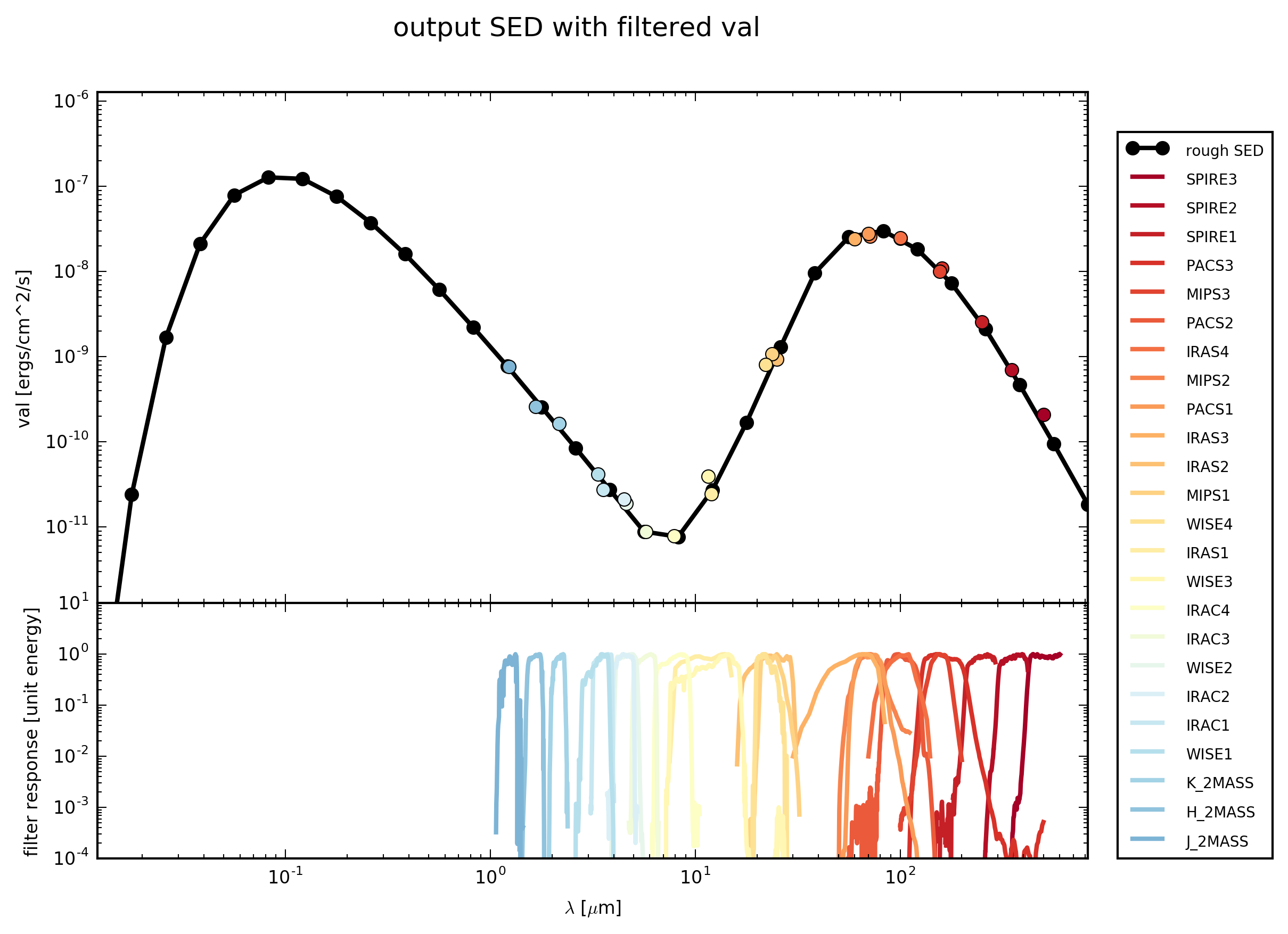
In this case you will find the file test_cube_process-output_SS-multi-filter.png in the directory where you run this script. If you extend the example described in SyntheticCube, the resulting image will be exactly the same as displayed below.

Of course you can add more things to the pipeline (resolution, extinction, PSF convolution, noise, ...) before you store the flux val in the arrays.