Convolve with PSF
By including the effects of diffraction at the opening of your artificial telescope the synthetic observation becomes more realistic.
With
fluxcompensator.cube.SyntheticCube.convolve_psf()fluxcompensator.image.SyntheticImage.convolve_psf()
you can convolve a physical property val of
- 3D (x, y, wav)
- 2D (x, y)
dimension of the different FC_objects, respectively, with a PSF of your choice. You can either convolve with a Gaussian PSF, an arbitrary function or with a file (e.g. provided from a certain telescope).
In any case add to your script:
# convolve with PSF
psf = FC_object.convolve_psf(psf_object)
By choosing from the three following options
you set up the object_psf and convolve your FC_object with it.
Warning
convolve_psf will not work for objects of SyntheticSED or SyntheticFlux.
Example: Plots
In what follows the convolution with FilePSF, FunctionPSF and GaussianPSF is presented. For comparison to FilePSF with the two other methods a PACS1 like PSF was produced and convolved with the synthetic reference image. For the setup see the subsections above.
Note
Here, for illustration purpose the almost the same PSF array was used to convolve the image. The different classes however, can be used to create any arbitrary PSF you might want to convolve the image with.
If the FC_object is a SyntheticCube, you can produce an image output by following the instruction Image Plots.
The essentials are given here; when the psf_object is a FilePSF add to your script
# psf_object is FilePSF
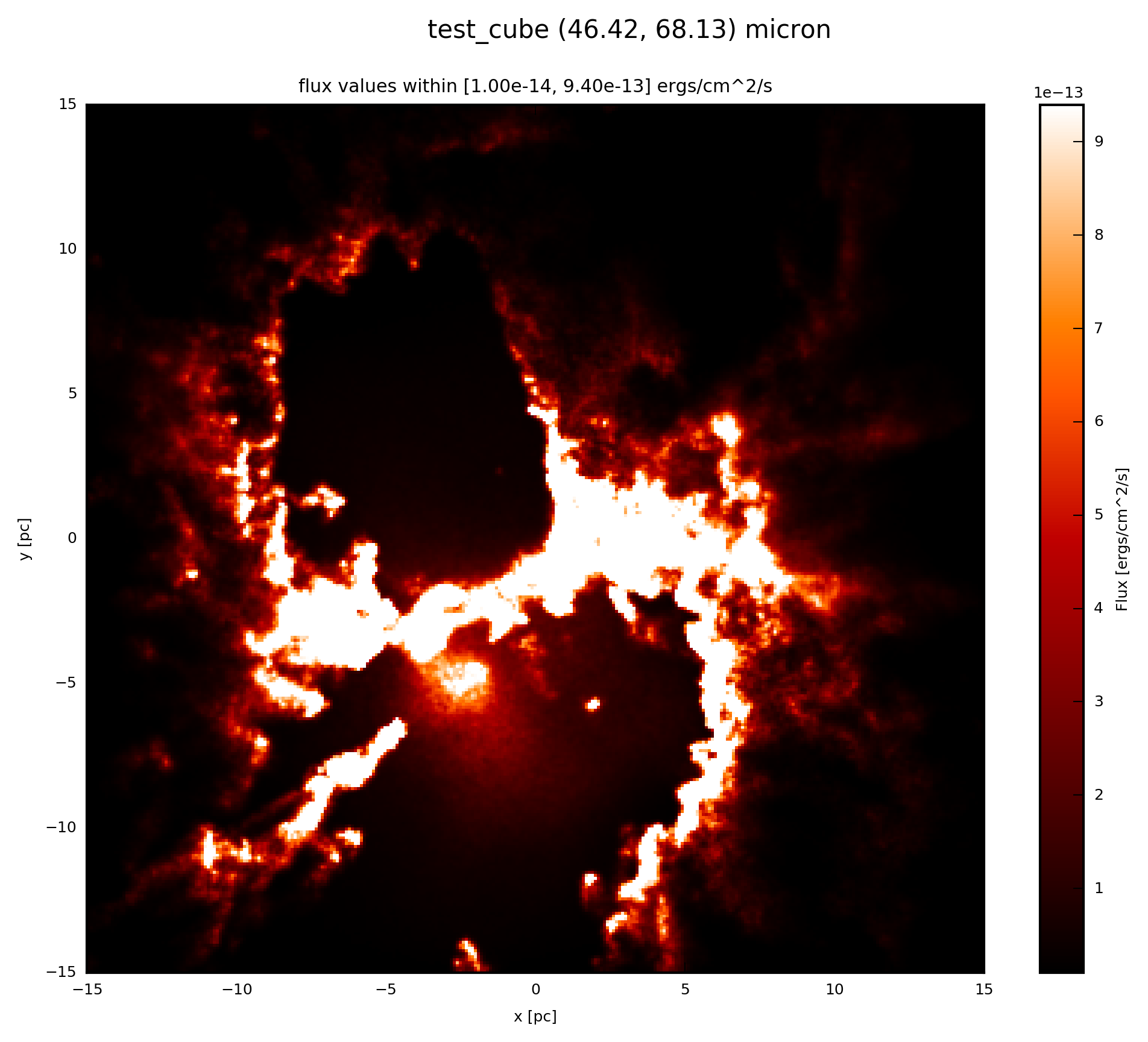
# plot psf.val (3D) at 60 microns
psf.plot_image(name='psf_file', wav_interest=60., set_cut=(1e-14, 9.4e-13),
single_cut=None, multi_cut=None, dpi=300)
In this case you will find the file test_cube_image_psf_file_set_cut_1.00e-14_9.40e-13_46.42_68.13.png in the same directory as example.py. If you extend the example described in SyntheticCube, the resulting image will be exactly the same as displayed below.

When the psf_object is a FunctionPSF add to your script:
# psf_object is FunctionPSF

# plot psf.val (3D) at 60 microns
psf.plot_image(name='psf_func', wav_interest=60., set_cut=(1e-14, 9.4e-13),
               single_cut=None, multi_cut=None, dpi=300)
In this case you will find the file test_cube_image_psf_func_set_cut_1.00e-14_9.40e-13_46.42_68.13.png in the same directory as example.py. If you extend the example described in SyntheticCube, the resulting image will be exactly the same as displayed below.

When the psf_object is a GaussianPSF add to your script:
# psf_object is GaussianPSF

# plot psf.val (3D) at 60 microns
psf.plot_image(name='psf_gauss', wav_interest=60., set_cut=(1e-14,
               9.4e-13), single_cut=None, multi_cut=None, dpi=300)
In this case you will find the file test_cube_image_psf_gauss_set_cut_1.00e-14_9.40e-13_46.42_68.13.png in the same directory as example.py. If you extend the example described in SyntheticCube, the resulting image will be exactly the same as displayed below.
Note
Here no change_resolution was used for illustration purposes. It might be however wise to use this tool.
If the FC_object is a SyntheticImage, because it was already convolved with a filter before, you plot with the following:
# plot psf.val (2D) at psf.wav
psf.plot_image(name='psf', set_cut=(1e-14, 9.4e-13), single_cut=None,
               multi_cut=None, dpi=300)
In this case you will find the file test_cube_image_psf_set_cut_1.00e-14_9.40e-13_*.png in the same directory as example.py, where * stands for the filter limits.