Adding of Noise
Gaussian noise can be added in order to account for random background.
With
you can add random noise to a synthetic measurement val with
- 3D (x, y, wav)
- 2D (x, y)
dimesion for the different FC_objects, respectively.
Note
In case of a 3D SyntheticCube different noise is added to every slice.
In any case add to your script:
# add noise
noise = FC_object.add_noise(mu_noise=0, sigma_noise=1e-13, seed=2, diagnostics=None)
The mu_noise and sigma_noise are given in the same units as the enteries of the image(s). If diagnostics=True an output of the noise will be created with the name test_cube_process-output_SC-noise.fits. Here you can see an example.
Warning
add_noise will not work for objects of SyntheticSED or SyntheticFlux.
Example: Plot
If the FC_object is a SyntheticCube, you can produce an image output by following the instruction Image Plots.
The essentials are given here; add to your script:
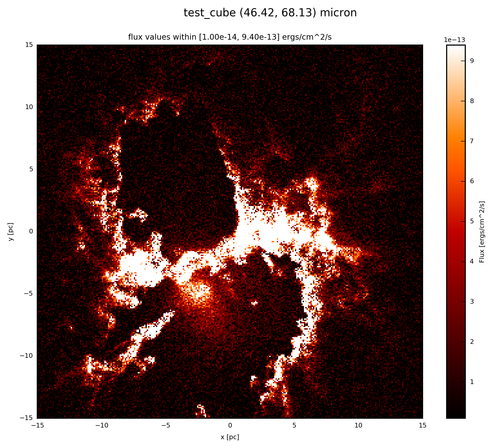
# plot noise.val at 60 microns
noise.plot_image(name='noise', wav_interest=60., set_cut=(1e-14, 9.4e-13),
                 single_cut=None, multi_cut=None, dpi=300)
In this case you will find the file test_cube_image_noise_set_cut_1.00e-14_9.40e-13_46.42_68.13.png in the same directory as example.py. If you extend the example described in SyntheticCube, the image will be similar the following.
Note
The plot is not exactly the same at the previous cases, since we used random noise. Only if you fixed it with the seed option.
If the FC_objects is a SyntheticImage, because it was already convolved with a filter before, you plot with the following:
# plot noise.val (2D) at noise.wav
noise.plot_image(name='noise', set_cut=(1e-14, 9.4e-13), single_cut=None,
                 multi_cut=None, dpi=300)
In this case you will find the file test_cube_image_noise_set_cut_1.00e-14_9.40e-13_*.png in the same directory as example.py, where * stands for the filter limits.