Resolution
The initial resolution of the physical property val in the FC_objects is set user through the distance setting in the ModelOutput, as well as the set_image_size and set_image_limits in the image set-up of Hyperion. However you can change the resolution also after the radiative transfer calculation (e.g. to compare with a certain observation or to convolve afterwards with a PSF from telescope specific a file).
Note
It is always useful to adjust the resolution of the FC_object to the resolution of the mimiced detector (e.g. PACS1).
With
fluxcompensator.cube.SyntheticCube.change_resolution()fluxcompensator.image.SyntheticImage.change_resolution()
you can change the resolution of val of
- 3D (x, y, wav)
- 2D (x, y)
dimension in the different FC_objects, respectively. In both cases add to your script:
# change resolution
zoom = FC_object.change_resolution(new_resolution=6., grid_plot=True)
new_resolution is the wanted resolution in arcsec/pixel. grid_plot=True will plot the old and new grid.
Warning
change_resolution will not work for objects of SyntheticSED or SyntheticFlux.
The new resolution will be updated to the attribute resolution of the SyntheticCube or SyntheticImage. When changing the resolution in some cases the width of the images changes. Therefore the attribute FOV will be updated as well.
Example: Plot
If the FC_object is a SyntheticCube, you can produce an image output by following the instruction Image Plots.
The essentials are given here; add to your script:
# plot zoom.val (3D) at 60 microns
zoom.plot_image(name='zoom', wav_interest=60., set_cut=(1e-13, 9.4e-12),
                single_cut=None, multi_cut=None, dpi=300)
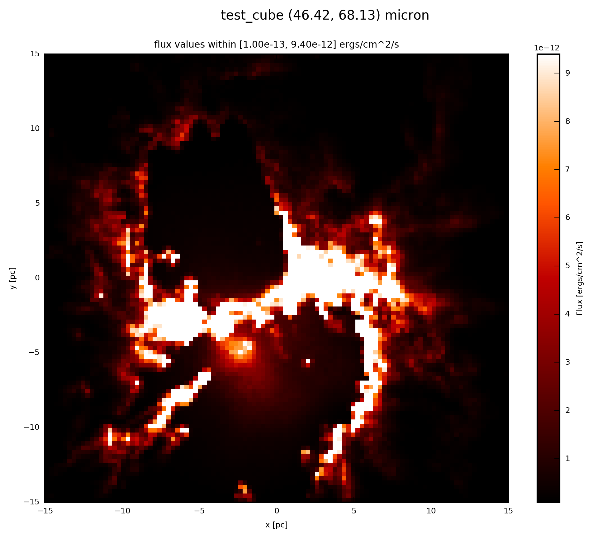
In this case you will find the file test_cube_image_zoom_set_cut_1.00e-13_9.40e-12_46.42_68.13.png in the same directory as example.py. If you extend the example described in SyntheticCube, the resulting image will be exactly the same as displayed below.
Note
The color bar limits on the right are different, here set_cut=(1e-13, 9.4e-12), because now several old pixels are joined compared to the initial image without resolution set_cut=(1e-14, 9.4e-13).
If the FC_object is a SyntheticImage, because it was already convolved with a filter before, you plot with the following:
# plot zoom.val (2D) at zoom.wav
zoom.plot_image(name='zoom', set_cut=(1e-13, 9.4e-12), single_cut=None,
                multi_cut=None, dpi=300)
In this case you will find the file test_cube_image_zoom_set_cut_1.00e-13_9.40e-12_*.png in the same directory as example.py, where * stands for the filter limits.